STATA Tutorial for Medical Research: Step-by-Step Guide for Beginners (2026)

Introduction

You finally get your hands on a research dataset, open it up, and now you don’t know what to do. If that blank-stare moment sounds familiar, STATA is worth a look. It’s a statistical software package made for crunching data, and over the years, it’s built up a devoted crowd in medicine.

No matter which research department you storm in, STATA’s in there somewhere. The reason clinicians keep coming back to it is simple enough: it chews through heavy analysis without a lot of drama, which counts for a lot when you’ve already got patients and paperwork pulling at you.

Whether you’re a student, a resident, or someone who’s been doing this for years, learning STATA is a skill that keeps paying off. This STATA tutorial for medical research takes you through the basics one piece at a time, until STATA software and medical statistics stop feeling like a wall.

What Is STATA and Why Is It Used in Medical Research?

At its core, STATA is a statistical software package for managing data, running tests, and figuring out what your results actually mean. Picture one tidy workspace where your dataset and your analysis sit right next to each other.

In medicine, you’ll bump into it almost everywhere. It drives clinical research, sifts through epidemiology data, and props up public health studies. Looking back at old records in a retrospective study? It does that. Following patients forward in a prospective one? That too. And in biostatistics, it’s a fixture.

Now, the obvious question: why not just stick with a spreadsheet? Excel is great for parking your numbers somewhere, but ask it to do real statistics, and it buckles fast. STATA runs the advanced tests, logs every move you make, and shrugs off huge datasets that would choke a spreadsheet. That kind of dependability is exactly what medical research can’t do without.

How to Install STATA and Set Up Your Workspace

Honestly, getting going is easier than people expect. STATA is licensed software, so the routine is to download it from the official site, run the installer, and punch in your license key. More often than not, your university or institution handles the access side for you.

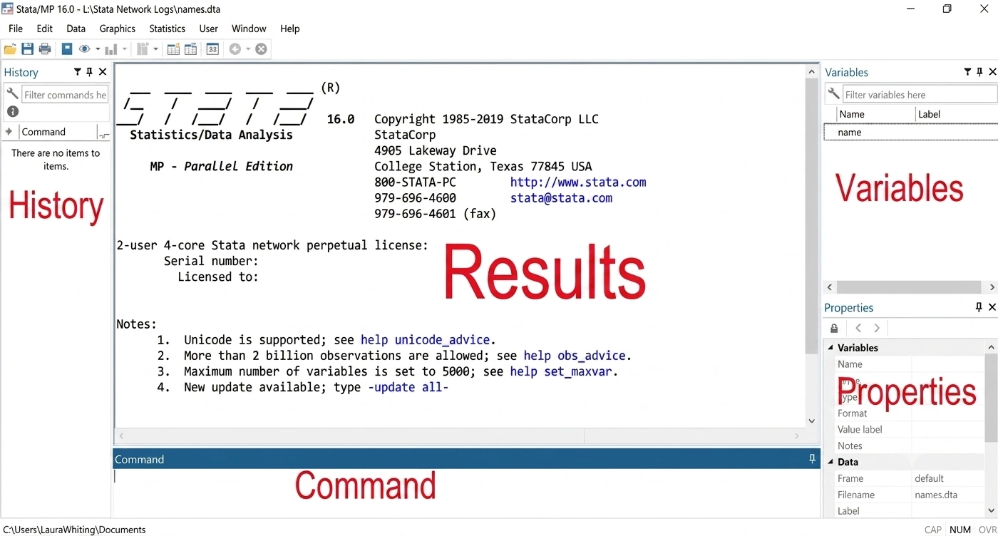
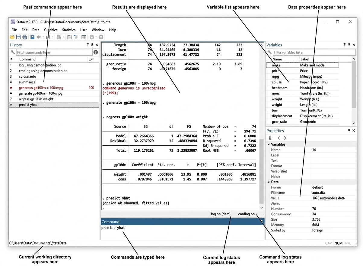
Open it up, and a handful of areas greet you. You type your instructions into the Command Window. Output lands in the Results Window. Everything in your dataset shows up in the Variables Window. And the Do-file Editor is where you save those commands as a script.

Pay attention to that last one. Do-files keep your analysis saved, repeatable, and easy to pass along to someone else. Build the habit now and thank yourself later.

That’s how the STATA interface looks

Importing Medical Research Data into STATA

None of the fun starts until your data is actually inside STATA, and the good news is the program isn’t picky about file types. Loads of medical data begins life in an Excel or CSV file. Using REDCap? Those exports drop right in. Even data scraped from electronic health records usually shows up in one of these formats first.

The routine itself is short. Import the dataset, save it as a STATA file, then give it a once-over to be sure nothing got mangled along the way.

Three commands earn their keep here:

• describe hands you a summary of your variables
• browse opens the data in a familiar spreadsheet-style view
• list prints rows straight into the results window

Pulling in that Excel file is usually a quick trip through the File menu, followed by a fast describe just to confirm everything landed where it should.

Data Cleaning and Management in STATA

Raw data almost never walks in ready to go. Something’s always a little off, and tidying it up first is what keeps you from chasing bad results down the road. This is the stage where you track down missing values, catch the duplicate records that slipped in twice, fix messy variables, and spin up new ones from what’s already sitting there.

A small set of commands carries most of the load:

• generate makes a brand-new variable
• replace updates the values in one you already have
• rename swaps in a clearer name
• drop clears out variables or records you don’t want

Picture it in action. Maybe you’d rather sort patients into age groups than work with exact ages. You’d lean on generate to build that grouping variable. BMI works the same way. Pull height and weight together, calculate BMI, then generate again to slot patients into underweight, normal, overweight, and obese buckets.

Tidy data today, answers you can trust tomorrow.

Descriptive Statistics in STATA

Before you touch a single fancy test, get a feel for what you’re working with. That’s the whole point of descriptive statistics, and STATA spits them out fast.

With numerical variables like age or blood pressure, you’re typically chasing the mean (the average), the median (the value in the middle), the standard deviation (how spread out everything is), and the range (lowest to highest). Categorical variables, think gender or smoking status, are a different story. There you want frequencies and percentages.

Two commands cover nearly all of it:

• summarize takes care of your numerical variables
• tabulate breaks the categorical ones into counts and percentages

Just about every study kicks off by describing the patients. Run a quick summarize on age, follow it with a tabulate on gender, and you’ve got a clean snapshot of who’s in your sample exactly the thing reviewers expect to see right at the top.

Performing Common Statistical Tests in STATA

With clean data in hand, this is where it gets interesting. STATA runs all the bread-and-butter tests of medical research, and most of the skill is just pairing the right test with the question you’re asking.

Comparing means. Two separate groups, like blood pressure in men versus women? That’s an independent t-test, and the command is ttest. But when those two readings come from the same patients before and after a treatment, say you switch to a paired t-test, still ttest, just with the paired option.

Comparing proportions. When both variables are categorical, like asking whether smoking ties to lung disease, the chi-square test is your tool. Run it with tabulate and the chi2 option.

Correlation analysis. Want to know if two variables rise and fall together, say age and cholesterol? Pearson correlation (correlate) handles normal data, while Spearman correlation (spearman) is your pick when the data is skewed.

Regression analysis. Linear regression predicts a number. Blood pressure from age and weight, for instance, using regress. Logistic regression predicts a yes-or-no outcome, like disease versus no disease, using logistic.

Stuck on which test to pick? Look at your outcome type first. That one decision usually walks you straight to the right command.

Creating Tables and Graphs in STATA

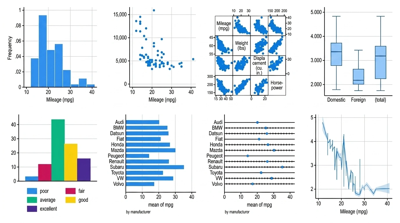
Numbers carry the story, sure, but a sharp graph is what makes people actually pay attention. STATA builds all the visuals you’re likely to reach for. Histograms lay out how one variable is spread. Bar charts stack groups side by side. Scatter plots expose the link between two variables, and box plots put spread and outliers on full display.

And there’s a real payoff here, not just decoration. Good visuals make your findings far easier to read, plus they hand you the publication-ready figures journals want. Most come from short commands, histogram, graph bar, scatter so making graphs in STATA is rarely more than a line or two.

How to Interpret STATA Output Correctly

Running the test? That’s the easy bit. Making sense of what comes back is where the real work lives. A few numbers do most of the heavy lifting.

The p-value flags whether your result is probably real or just luck, and anything under 0.05 usually gets the “significant” label. The confidence interval marks out the range your true value most likely falls in. Odds ratios, the regulars of logistic regression, show how much something bumps the odds of an outcome up or down. And regression coefficients tell you how far your outcome moves when a predictor shifts.

Beginners tend to stumble into two pits. One is treating a significant p-value like proof that something matters. The other is the opposite mistake, brushing off clinical significance. A difference can be statistically significant and still mean absolutely nothing for a real patient. Keep both lenses on when you read your numbers.

Common STATA Errors and How to Fix Them

Those red error messages hit everybody, so there’s no need to flinch when one lands. A handful show up over and over. “Variable not found” is nearly always a typo or a capital letter where you meant lowercase. A type mismatch crops up when you treat text like a number, or flip it the other way. Missing values can throw a command off without warning, too. And syntax errors? Nine times out of ten it’s a comma in the wrong spot. The cure barely changes: read the message, double-check your spelling, and glance at the line just above where it quit.

Conclusion

And that’s the tour. You’ve walked through importing your data, scrubbing it clean, pulling descriptive statistics, running the core tests, and reading your output without flinching at every figure. That’s a genuinely solid base to keep building on.

The real growth, though, comes once you start messing around with actual datasets. Grab one from your own work and tinker. Every bit of practice makes you quicker and steadier, and that shows up directly in your research and your publication track record.

No matter what statistical software you want to learn, it is important that you learn the basics of biostatistics. If you are a beginner, and want to learn biostats from scratch, American Academy of Research and Academics is the right place for you. Enroll in our course today to start your learning journey.